Motor Trend Regression Models

Introduction

Motor Trend, is a magazine about the automobile industry. The data was extracted from the 1974 Motor Trend US magazine, and comprises fuel consumption and 10 aspects of automobile design and performance for 32 automobiles (1973-74 models). They are particularly interested in the following two questions:

1. Is an automatic or manual transmission better for MPG.
2. Quantify the MPG difference between automatic and manual transmissions.

Loading required libraries

# Required libraries
library(ggplot2)
library(psych)
library(MASS)

Load Data and Preprocessing

data(mtcars)
mtcars$am <- factor(mtcars$am,labels=c('Automatic','Manual'))

Perform some basic exploratory data analyses

Let us see how response variable MPG correlate with all the explanatory variables.

pairs.panels(mtcars, main="Pair Graph of Motor Trend Car Road Tests")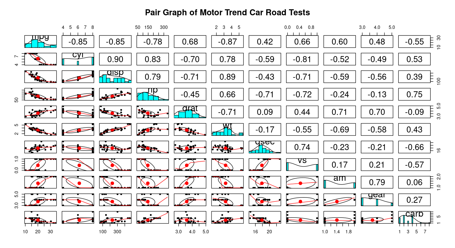

The pairs plot show us correlation between different variables. This will be useful once we find out model.

plotbox(mtcars)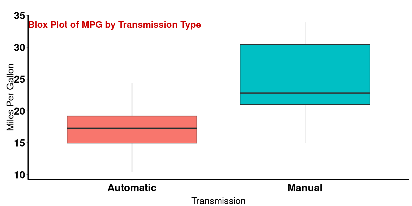

Inference

Next, my hypothesis question: Is there a difference between the average MPG for mtcars using manual transmission and those using automatic transmission.

(mpg <- t.test(mpg ~ am,mtcars))
paste("For Manual and Automatic p-value is",
      format(mpg$p.value, scientific=FALSE), ":reject NULL hypothesis", sep=" ")

## 
##  Welch Two Sample t-test
## 
## data:  mpg by am
## t = -3.7671, df = 18.332, p-value = 0.001374
## alternative hypothesis: true difference in means is not equal to 0
## 95 percent confidence interval:
##  -11.280194  -3.209684
## sample estimates:
## mean in group Automatic    mean in group Manual 
##                17.14737                24.39231 
## 
## [1] "For Manual and Automatic p-value is 0.001373638 :reject NULL hypothesis"

Regression Analysis

In linear regression we estimate two parameter: \(\beta_{0}\) and \(\beta_{1}\). So we lose 1 degree of freedom for each parameter as penalty. So k is the number of degrees of freedom. AIC: k = 2. BIC: k = \(\log_{n}\).

Adjusted \(R^2\) vs P-value:

• p-value - when interested in finding out which predictor are statistically significant
• adjusted \(R^2\) - when interested in a more reliable predictors.

I am going to use adjusted \(R^2\) to pick my final model.

Backward elimination method begins with the full model, drop one variable at a time and record adjusted \(R^2\) of each smaller model. Pick the model with the highest increase in adjusted \(R^2\).

Forward selection method starts with single predictor of response vs. each explanatory variable. Add the remaining variables one at a time to existing model and pick the model with highest adjusted \(R^2\).

I decided to use stepAIC function from the MASS package to perform this analysis because it is automated. However, I will include non-automated linear fit using AIC and BIC to see if we get same best/final models.

#All Results hidden
AutoFullModel <- stepAIC(lm(mpg ~ . ,data=mtcars), 
                         direction = 'both', k = log(32), trace = FALSE)
ManualFullModel <- lm(mpg ~ ., data=mtcars)
forwardModelAIC <- step(lm(mpg ~ 1, data = mtcars), 
      direction = "forward", scope = formula(ManualFullModel), k = 2, trace = 0)
forwardModelBIC <- step(lm(mpg ~ 1, data = mtcars), 
      direction = "forward", scope = formula(ManualFullModel), k = log(32), trace = 0)
backwardModelAIC <- step(ManualFullModel, 
      direction = "backward", k = 2, trace = 0)
backwardModelBIC <- step(ManualFullModel, direction = "backward", k = log(32), trace = 0)

Below are the Automated MASS package results:

AutoFullModel$anova

## Stepwise Model Path 
## Analysis of Deviance Table
## 
## Initial Model:
## mpg ~ cyl + disp + hp + drat + wt + qsec + vs + am + gear + carb
## 
## Final Model:
## mpg ~ wt + qsec + am
## 
## 
##     Step Df   Deviance Resid. Df Resid. Dev      AIC
## 1                             21   147.4944 87.02084
## 2  - cyl  1 0.07987121        22   147.5743 83.57243
## 3   - vs  1 0.26852280        23   147.8428 80.16486
## 4 - carb  1 0.68546077        24   148.5283 76.84715
## 5 - gear  1 1.56497053        25   150.0933 73.71682
## 6 - drat  1 3.34455117        26   153.4378 70.95632
## 7 - disp  1 6.62865369        27   160.0665 68.84398
## 8   - hp  1 9.21946935        28   169.2859 67.17025

Below are adjusted \(R^2\) results non-automated linear models fitted using AIC and BIC:

formulafAIC <- toString(c(summary(forwardModelAIC)$call$formula))
msg<-paste("Forward AIC highest Adjusted $R^2$ value of",
  format(summary(forwardModelAIC)$adj.r.squared),"and that model is",formulafAIC,sep=" ")
formulafBIC <- toString(c(summary(forwardModelBIC)$call$formula))
msg1<-paste("Forward BIC highest Adjusted $R^2$ value of",
  format(summary(forwardModelBIC)$adj.r.squared),"and that model is",formulafBIC,sep=" ")
formulabAIC <- toString(c(summary(backwardModelAIC)$call$formula))
msg2<-paste("Backward AIC highest Adjusted $R^2$ value of",
  format(summary(backwardModelAIC)$adj.r.squared),"and that model is",formulabAIC,sep=" ")
formulabBIC <- toString(c(summary(backwardModelBIC)$call$formula))
msg3<-paste("Backward BIC highest Adjusted $R^2$ value of",
  format(summary(backwardModelBIC)$adj.r.squared),"and that model is",formulabBIC,sep=" ")
prnt.test(c(msg,msg1,msg2,msg3))

Forward AIC highest Adjusted \(R^2\) value of 0.8263446 and that model is mpg ~ wt + cyl + hp

Forward BIC highest Adjusted \(R^2\) value of 0.8185189 and that model is mpg ~ wt + cyl

Backward AIC highest Adjusted \(R^2\) value of 0.8335561 and that model is mpg ~ wt + qsec + am

Backward BIC highest Adjusted \(R^2\) value of 0.8335561 and that model is mpg ~ wt + qsec + am

As you can see the non-automated linear fit best model based on the adjusted \(R^2\), is: . It is the same as the automated linear fit using MASS package.

Now we go back to the pairs plot. We observe that wt and am have a negative correlation of -69. As a result we will have to include that interaction in our custom final model: .

Residual Analysis and Diagnostics

Diagnostic for Multiple Linear regression has the following items:

• How is response variable linearly related to the explanatory variable.
• Nearly normal residuals with mean of zero.
• Constant variability of residual.
• Independence of residuals.

customFinalModel<-lm(mpg ~ wt + qsec + am + wt:am, data=mtcars)
par(mfrow = c(2, 2))
plot(customFinalModel)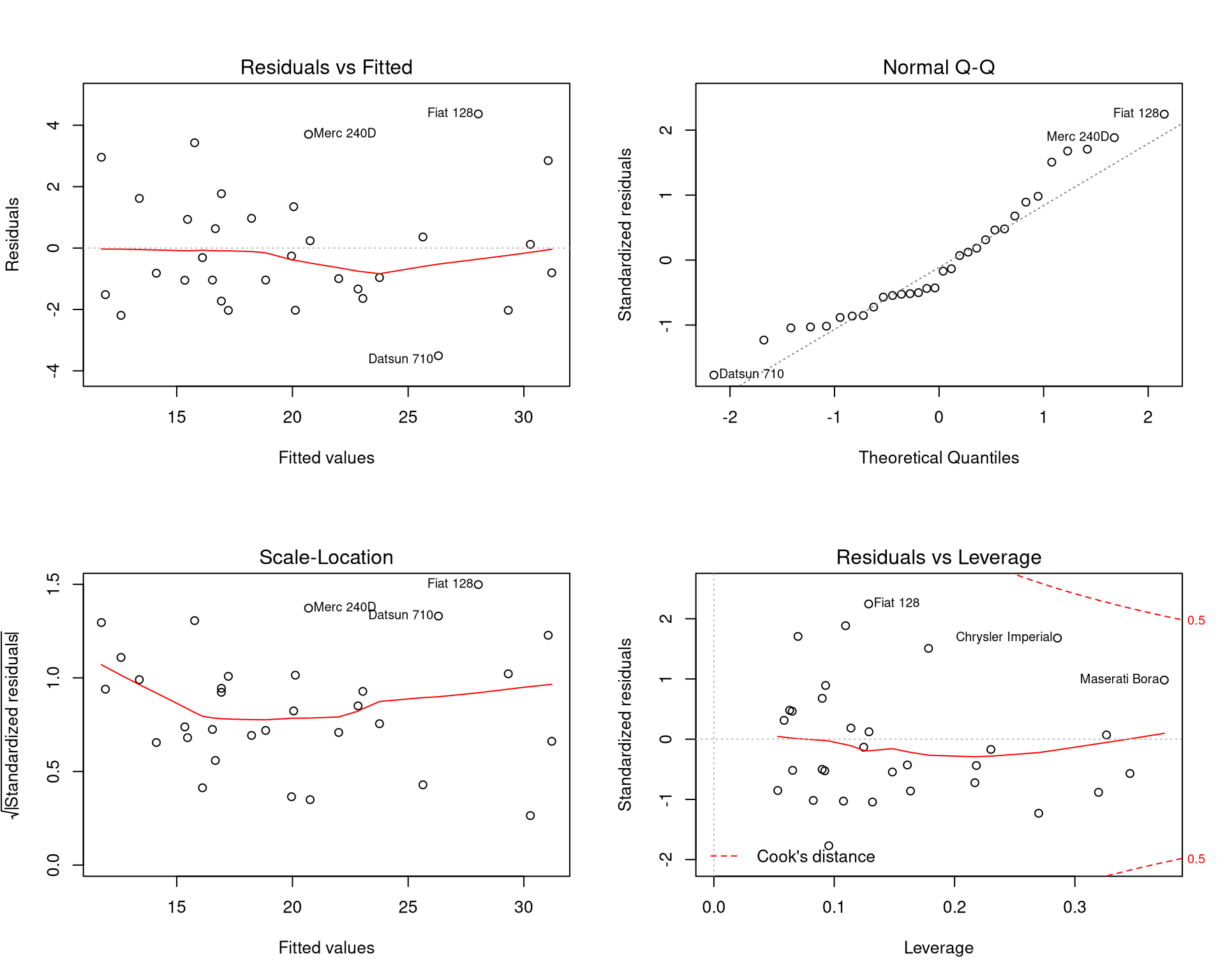

• Residual vs Leverage: we observe no outliers. All cases are inside dashed line, Cook’s distance.
• Normal Q-Q Plot: we observe that residual plot is nearly normal centered around 0.
• Scale-Location: we observed that plots of vs. randomly scatter in a band with a constant width around 0 (no fan shape).
• Residual vs Fitted: we observe a residual plot that has no pattern(complete random scatter).

R Code

#Function for plotting histogram and Printing function
plotbox <- function(box.data){
  ggplot(box.data,aes(x=factor(am),y=mpg, fill=am))+geom_boxplot()+labs(x="X (binned)")+
  theme(axis.text.x=element_text(angle=0, vjust=0.4,hjust=0.5,face="bold",
                                 color ="black", size =rel(2)),
        axis.title.x = element_text(size = rel(1.5),vjust= -.5),
        axis.text.y = element_text(face="bold", color="black", size =rel(2)),
        axis.title.y = element_text(size = rel(1.5), angle = 90,vjust=-.5),
        strip.text.x = element_text(size=rel(2),face="bold"),
        legend.position = "none", panel.grid.major = element_blank(),
        panel.background = element_rect(fill = "transparent"),
        axis.line = element_line(colour = "black", size=1, linetype = "solid"),
        plot.title = element_text(vjust=-8,lineheight=.8, face="bold",
                                  color="#CD0000", size=16))+
  scale_x_discrete("Transmission") + scale_y_continuous("Miles Per Gallon") + 
  ggtitle("Blox Plot of MPG by Transmission Type")
}
prnt.test <- function(x){cat(x, sep="\n\n")}