Part 1 Statistical Inference

Introduction

In this project you will investigate the exponential distribution in R and compare it with the Central Limit Theorem. The exponential distribution can be simulated in R with rexp(n, \(\lambda\)) where lambda(\(\lambda\)) is the rate parameter. The mean of exponential distribution is 1/\(\lambda\) and the standard deviation is also 1/\(\lambda\). Set \(\lambda\) = 0.2 for all of the simulations. You will investigate the distribution of averages of 40 exponentials. Note that you will need to do a thousand simulations

Loading required libraries

# Required libraries
library(ggplot2)

Simulation Data and Preprocessing

# set constants
lambda <- 0.2 # lambda for rexp
n <- 40 # exponentials
simCount <- 1000 # number of simulations
# set the seed to create reproducability
set.seed(02122016)


# run the test resulting in n x SimCount matrix
expSimSample <- matrix(rexp(n * simCount, lambda), nrow=simCount)
expSimSampleMeans <- apply(expSimSample, 1, mean)

Sample Mean versus Theoretical Mean

Sample mean \((\bar{X})\) from the simulation sample

mean(expSimSample)

## [1] 5.031448

The theoretical mean \(\mu\) of a exponential distribution of rate \(\lambda\) is

\(\mu= \frac{1}{\lambda}\)

(mu <- 1/lambda)

## [1] 5

Sample mean \((\bar{X})\) and the theoretical mean \(\mu\) are very close.

Sample Variance versus Theoretical Variance

Sample variance \(s^2\) from the simulation sample means

#The var function calculates population variance
(samplevar <-var(expSimSampleMeans))

## [1] 0.6404317

The theoretical standard deviation \(\sigma\) of a exponential distribution of rate \(\lambda\) is

\(\sigma = \frac{1/\lambda}{\sqrt{n}}\)

The theoretical variance \(\sigma^2\) of a exponential distribution of rate \(\lambda\) is

\(\sigma^2 = (\frac{1/\lambda}{\sqrt{n}})^2\)

(sd <- 1/lambda/sqrt(n))
(var <- sd^2)

## [1] 0.7905694
## [1] 0.625

[1] “As you can see, the sample variance of is 0.64 which is also close the theoretical variance 0.625 .”

Show that the distribution is approximately normal

plotdist(expSimSampleMeans, mu)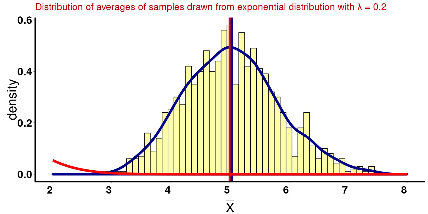

The graph shows the sample mean and its distribution(blue line). It is approximately normal compared to the theoretical mean of the exponential distribution based on the given lamba. This example validates the Centrai Limit Theorem.

Appendix

#Function for plotting histogram
plotdist <- function(bar.data, mu){
  ggplot(data.frame(bar.data), aes (x = bar.data)) + 
  geom_histogram(aes(y = ..density..), colour = "#000000", 
                 fill = "#FFFFAA", binwidth=0.1) + 
  geom_density(colour = "darkblue", size =rel(2)) +
  geom_vline(xintercept = mu, size = rel(2),colour = "red") +
  geom_vline(xintercept = mean(bar.data), size = rel(2),
             colour = "darkblue") +
  xlab(expression(bar(X))) + 
  ggtitle(expression(paste("Distribution of averages of samples",
                           " drawn from exponential distribution with ",
                           lambda, " = 0.2", sep = " "))) +
  theme(axis.text.x = element_text(angle = 0, hjust = 1, vjust=.5,
                                   face="bold", color ="black", size =rel(2)),
        axis.title.x = element_text(size = rel(2),vjust= -.5),
        axis.text.y = element_text(face="bold", color="black", size =rel(2)),
        axis.title.y = element_text(size = rel(2), angle = 90,vjust=-.2),
        panel.grid.major = element_blank(), 
        panel.grid.minor = element_blank(), 
        panel.background = element_rect(fill = "transparent"),
        axis.line = element_line(colour = "black", size=1, linetype = "solid"),
        plot.title = element_text(vjust= 1,lineheight=.8, face="bold",
                                  color="#CD0000", size=16))+
  scale_x_continuous(breaks=seq(mu-3,mu+3,1), limits=c(mu-3,mu+3))+
  stat_function(fun = dnorm, arg = list(mean = mu, sd = sd),
                colour = "red", size =rel(2))
}